Decision Tree in Machine Learning
What are Machine Learning Algorithms?
Algorithms are step-by-step computational procedures for solving a problem, similar to decision-making flowcharts, used for information processing, mathematical calculation, and other related operations.
Basics of decision tree algorithm
Introduction to decision tree
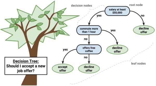
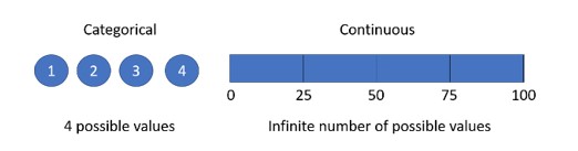
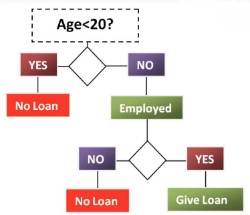
Decision Tree is a type of Supervised Learning Algorithm (i.e. you explain what the input is and what the corresponding output is in the training data) that can be used for solving regression and classification problems by using tree representation. Decision trees can handle both categorical and continuous data. The tree can be explained by two entities, namely decision nodes and leaf nodes. The leaf nodes are the decisions or the final outcomes (categorical or continuous value) and each leaf node corresponds to a class label. The decision nodes or internal nodes are where the data is split (has two or more branches) and each internal nodes of the tree corresponds to an attribute. The topmost decision node in a tree which corresponds to the best predictor is call called the root node.
There are two main types of Decision Trees:
1. Classification trees (Yes/No types)
What we’ve seen above was an example of a classification tree, where the outcome was a variable like ‘accept offer’ or Decline offer. Here the decision variable is Categorical.
2. Regression trees (Continuous data types)
Here the decision or the outcome variable is Continuous and is considered a real number (i.e. a number like 1,2,3). Example of real numbers is price of a house or a patient's length of stay in a hospital
Use Case 01 - Analysis by making best efforts to process the analytics data to identify business queries and visualize data with AWS based BI tools.
Use Case 02 - Build a predictive model that leverages the AWS ML and associated services using the available Adobe Analytics data and make business decisions using a ML model.
How to build this??
There are many specific decision-tree algorithms to build a decision tree.
Here we only talk about a few which are,
ID3 (Iterative Dichotomiser 3) Algorithm
ID3 (Iterative Dichotomiser 3) is one of the most common decision tree algorithm introduced in 1986 by Ross Quinlan. The ID3 algorithm builds decision trees using a top-down, greedy approach and it uses Entropy and Information Gain to construct a decision tree. Before discussing the ID3 algorithm, we’ll go through a few definitions.
Entropy
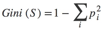
Entropy, also called as Shannon Entropy is denoted by H(S) for a finite set S, is the measure of the amount of uncertainty or randomness in data.
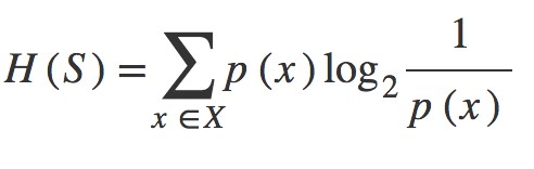
S - The current (data) set for which entropy is being calculated (change every iteration of the ID3 algorithm)
x - Set of classes in S x={ yes, no }
p(x) - The proportion of the number of elements in class x to the number of elements in set S
Given a collection S containing positive and negative examples of some target concept, the entropy of S relative to this boolean classification is:
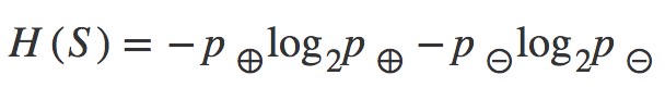
For a binary classification problem with only two classes, positive and negative class.
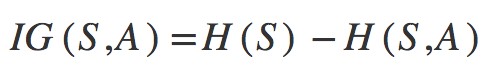
Information Gain
Information gain is also called as Kullback-Leibler divergence denoted by IG(S,A) for a set ‘S’ is the effective change in entropy after deciding on a particular attribute ‘A’. It measures the relative change in entropy with respect to the independent variables. IG(A) is the measure of the difference in entropy from before to after the set ‘S’ is split on an attribute ‘A’. In other words, how much uncertainty in ‘S’ was reduced after splitting set ‘S’ on attribute ‘A’. It decides which attribute goes into a decision node. To minimize the decision tree depth, the attribute with the most entropy reduction is the best choice.
Alternatively
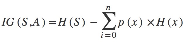
where,
IG(S, A) - information gain by applying feature A.
H(S) - Entropy of set S
T - The subset created from splitting S by attributing A such that
p(x) - The proportion of the number of elements in x to the number of elements in set S
H(x) - Entropy of subset x
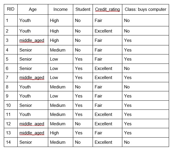
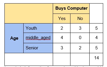
To get a clear understanding of calculating information gain & entropy, we will try to implement it on sample data. Consider a piece of data collected from a computer shop where the features are age, income, student, credit rating and the outcome variable is whether the customer buys a computer or not. Now, our job is to build a predictive model which takes in above 4 parameters and predicts whether the customer will buy a computer or not. We’ll build a decision tree to do that using ID3 algorithm.
ID3 Algorithm will perform following tasks recursively
1. Create a root node for the tree2. If all examples are positive, return leaf node ‘positive’
3. Else if all examples are negative, return leaf node ‘negative’
4. Calculate the entropy of current state H(S)
5. For each attribute, calculate the entropy with respect to the attribute ‘x’ denoted by H(S, x)
6. Select the attribute which has the maximum value of IG(S, x)
7. Remove the attribute that offers highest IG from the set of attributes
8. Repeat until we run out of all attributes, or the decision tree has all leaf nodes.
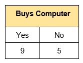
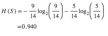
Step 1: The initial step is to calculate H(S), the Entropy of the current state. In the above example, we can see in total there are 5 No’s and 9 Yes’s.
Step 2 : The next step is to calculate H(S,x), the entropy with respect to the attribute ‘x’ for each attribute. In the above example, The expected information needed to classify a tuple in ‘S’ if the tuples are partitioned according to age is,
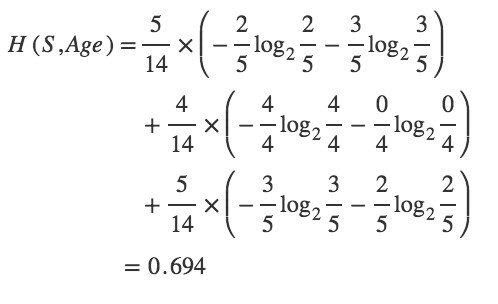
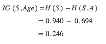
Hence, the gain in information from such partitioning would be,
Similarly,
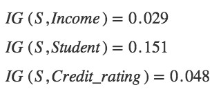
Step 3: Choose attribute with the largest information gain, IG(S,x) as the decision node, divide the dataset by its branches and repeat the same process on every branch. Age has the highest information gain among the attributes, so Age is selected as the splitting attribute.
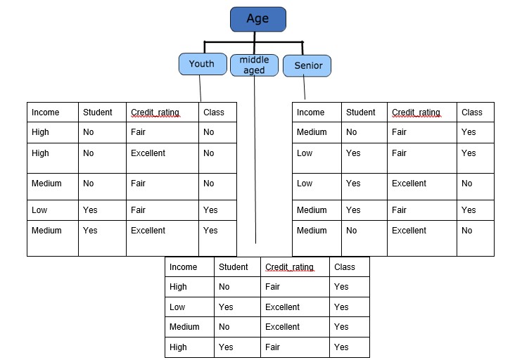
Step 4a: A branch with an entropy of 0 is a leaf node.
Step 4b : A branch with entropy more than 0 needs further splitting.
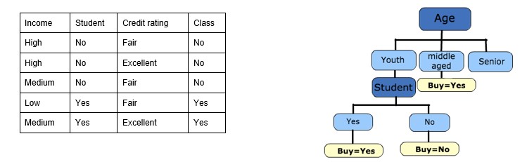
Step 5: The ID3 algorithm is run recursively on the non-leaf branches until all data is classified.
Decision Tree to Decision Rules
A decision tree can easily be transformed into a set of rules by mapping from the root node to the leaf nodes one by one.
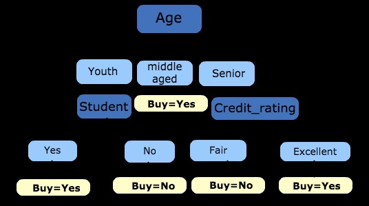
R1 : If (Age=Youth) AND (Student=Yes) THEN Buys_computer=Yes
R2 : If (Age=Youth) AND (Student=No) THEN Buys_computer=No
R3 : If (Age=middle_aged) THEN Buys_computer=Yes
R4 : If (Age=Senior) AND (Credit_rating=Fair) THEN Buys_computer=No
R5 : If (Age=Senior) AND (Credit_rating =Excellent) THEN Buys_computer=Yes
Pseudocode: ID3 is a greedy algorithm that grows the tree top-down, at each node selecting the attribute that best classifies the local training examples. This process continues until the tree perfectly classifies the training examples or until all attributes have been used. The pseudocode assumes that the attributes are discrete and that the classification is binary. Examples are the training example. Target_attribute is the attribute whose value is to be predicted by the tree. Attributes are a list of other attributes that may be tested by the learned decision tree. Finally, it returns a decision tree that correctly classifies the given Examples.
Advantages and Disadvantages of Decision Tree Algorithm
Advantages:
1. Decision Trees are easy to explain. It results in a set of rules.
2. It follows the same approach humans generally follow while making decisions.
3. Interpretation of a complex Decision Tree model can be simplified by its visualizations.
4. Decision trees can be used to predict both continuous and discrete values i.e. they work well for both regression and classification tasks.
5. They require relatively less effort for training the algorithm.
6. They can be used to classify non-linearly separable data.
7. Resistant to outliers, hence require little data preprocessing
8. They're very fast and efficient compared to KNN and other classification algorithms.
1. There is a high probability of overfitting in the Decision Tree.
2. Generally, it gives low prediction accuracy for a dataset as compared to other machine learning algorithms.
3. Information gain in a decision tree with categorical variables gives a biased response for attributes with greater no. of categories.
4. Calculations can become complex when there are many class labels.
Splitting
The process of partitioning the data set into subsets. Splits are formed on a particular variable
How to Specify Test Condition?
Splitting Based on Nominal Attributes
- Multi-way split: Use as many partitions as values
- Binary split: Divide values into two subsets

Splitting Based on Continuous Attributes
Different ways of handling- Multi-way split: form ordinal categorical attribute ◆ Static – discretize once at the beginning ◆ Dynamic – repeat on each new partition
- Binary split: (A < v) or (A ≥ v) ◆ How to choose v?
Need to find optimal partitioning!
Can use GAIN or GINI !
Pruning
The shortening of branches of the tree. Pruning is the process of reducing the size of the tree by turning some branch nodes into leaf nodes(opposite of Splitting), and removing the leaf nodes under the original branch. Pruning is useful because classification trees may fit the training data well, but may do a poor job of classifying new values. A simpler tree often avoids overfitting.
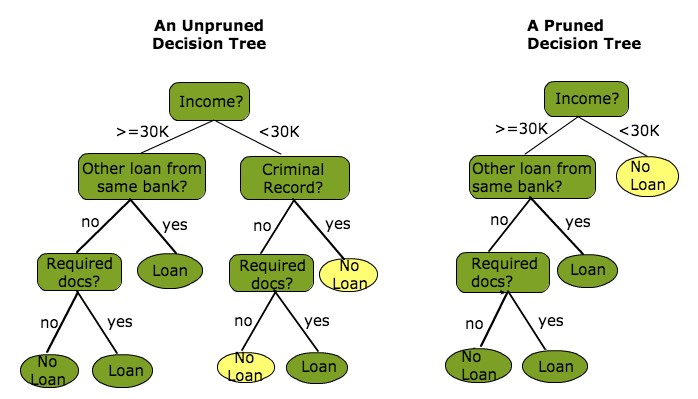
Overfitting
Overfitting is a practical problem while building a decision tree model. The model has an issue of overfitting when the algorithm continues to go deeper and deeper in to reduce the training set error, but results with an increased test set error i.e, reduces the accuracy of the prediction for our model. It generally happens when it builds many branches due to outliers and irregularities in data. Two approaches which we can use to avoid overfitting are:
Pre-Pruning
In pre-pruning, it stops the tree construction early. It is preferred not to split a node if its goodness measure is below a threshold value. But it’s difficult to choose an appropriate stopping point.
Post-Pruning
In post-pruning, first it goes deeper and deeper in the tree to build a complete tree. If the tree shows the overfitting problem then pruning is done as a post-pruning step. We use cross-validation data to check the effect of our pruning. Using cross-validation data, it tests whether expanding a node will make an improvement or not. If it shows improvement, then we can continue by expanding that node. But if it shows a reduction in accuracy then it should not be expanded i.e, the node should be converted to a leaf node.
CART (Classification And Regression Tree) Algorithm
Classification and Regression Trees or CART for short is a term introduced by Leo Breiman to refer to Decision Tree algorithms that can be used for classification and regression predictive modelling problems for numeric attributes (regression) or categorical attributes (classification). Decision tree models where the target variable can take a discrete set of values are called Classification Trees and decision trees where the target variable can take continuous values are known as Regression Trees. The representation for the CART model is a binary tree. In CART we use Gini index as a metric.
Gini Index
Steps to Calculate Gini for a split
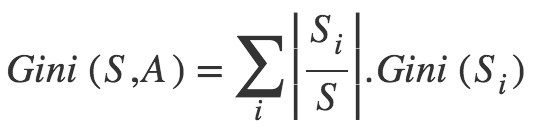
1.Calculate Gini for sub-nodes, using formula sum of square of probability for success and failure (p^2+q^2).
Calculate Gini for split using weighted Gini score of each node of that split.
CART steps
1. Start with the root node (all data in dataset)2. Split the node with minimum Gini Index Recursive process
3. Assign nodes with predicted classes
4. Missing data: program uses best available info to replace missing data (based on a variable that is relative to the outcome variable)
5. Stop tree building: when every aspect of the dataset is visible in decision tree
6. Tree Pruning: based on miscalculation rate
7. Optimal Selection: best tree that fit dataset with a low percentage of error
To get a clear understanding of calculating Gini index, we will try to implement it on the previous data set used in above ID3 algorithm.
Split on Age:
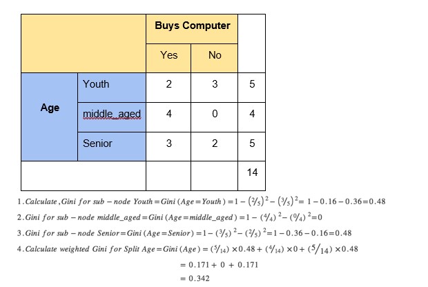
Similarly,
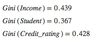
Choose attribute with the minimum Gini Index, Gini(S) as the decision node, divide the dataset by its branches and repeat the same process on every branch. Age has the minimum Gini Index among the attribute, so Age is selected as the splitting attribute.
Repeat until we run out of all attributes, or the decision tree has all leaf nodes.
NOTE: This does not mean that ID3 and CART algorithms produce the same trees always. References:1. Information Gain: https://en.wikipedia.org/wiki/Information_gain_in_decision_trees
2. Entropy: https://en.wikipedia.org/wiki/Entropy_(information_theory)
3. ID3: https://en.wikipedia.org/wiki/ID3_algorithm
4. ID3 Example: https://www.cise.ufl.edu/~ddd/cap6635/Fall-97/Short-papers/2.htm
5. Gini Index: https://en.wikipedia.org/wiki/Gini_coefficient
6. ID3 and CART: https://medium.com/deep-math-machine-learning-ai/chapter-4-decision-trees-algorithms-b93975f7a1f1
7. CART Example: https://sefiks.com/2018/08/27/a-step-by-step-cart-decision-tree-example/

Chamalka Gamaralalage
Associate Software EngineerDeveloping a Custom Audit Trail and a Notification Service for a Workflow Based Serverless Application on AWS
READ ARTICLE
Human Emotions Recognition through Facial Expressions and Sentiment Analysis for Emotionally Aware Deep Learning Models
READ ARTICLE